SMELT: Scaling Laws for Compute-Matched MoE Looped Transformers

Authoritative Technical Breakdown & Systems Analysis
Paper: SMELT: Scaling Laws for Compute-Matched MoE Looped Transformers (arXiv:2609.01343, September 2026)
Authors: Shaowen Wang, Ge Zhang, Kairong Luo, Yuhao Wu, Shaofan Liu, Jiaheng Liu, Wenhao Huang, Shen Yan, Jian Li
Affiliations: Tsinghua University, ByteDance Seed, M-A-P, TokenWave.AI

Executive Summary & Table of Contents

For years, Looped Transformers (from Universal Transformers to ALBERT and Huginn) promised a holy grail for LLM architectures: increasing effective model depth and algorithmic reasoning power by reusing a shared block of layer parameters, without bloating the physical model size stored on disk.

However, production ML researchers and inference engineers remained skeptical—and rightly so. Historical evaluations fell into what we term the FLOP-Inflation Conflation Trap:

Parameter-Fixed Benchmarking (The Trap): Repeating a 12-layer block to 24 executed layers kept stored parameters constant but secretly doubled per-token FLOPs and doubled KV cache memory footprint, misattributing raw extra compute to architectural ingenuity.
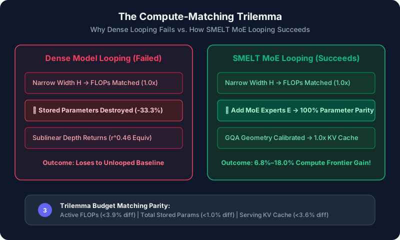
Iso-FLOP Shrinkage in Dense Models: When FLOPs were held fixed in dense architectures (e.g., Schwethelm et al.), narrowing the hidden dimension $d_{\text{model}}$ to pay for extra layer iterations permanently destroyed unique stored parameter capacity, resulting in sublinear capacity returns ( $r^{0.46}$ unique-block equivalence) that lost to unlooped baselines.

Enter SMELT (Sparse MoE Transformer, middle layers Loop Twice) by Shaowen Wang and the ByteDance Seed team. SMELT solves this decades-old architectural paradox by pairing middle-block layer looping with Sparse Mixture-of-Experts (MoE). Because MoE decouples total parameter capacity from active per-token FLOPs, SMELT pays for its extra layer passes by narrowing the hidden dimension $H$ , and fully recovers total parameter capacity by raising the total expert count $E$ .

1. Active Compute ( $C_{\text{token}}$ )	2. Stored Parameters ( $N_{\text{total}}$ )	3. Serving KV Cache ( $M_{\text{KV}}$ )
Strictly Matched ( $\le 3.9\%$ mismatch)	Strictly Matched ( $\le 1.0\%$ mismatch)	Matched Parity (GQA & Head Dim calibration)

Across a massive empirical scaling ladder (up to 54B non-embedding total parameters, 1.6B active non-embedding parameters, 4 scales $\times$ 4 sparsity levels), SMELT establishes that depth reuse yields a genuine 6.8%–18.0% compute efficiency gain on the Chinchilla scaling frontier, outperforming unlooped baselines on downstream benchmarks (DCLM Core, DCLM Completion, MMLU 5-shot, Code, and Long-Context ICL) beyond what aggregate validation loss alone predicts.

Executive 5W1H & High-Impact Hook
- 1.5 The Intuitive Mental Model: SMELT in Plain English (Zero Math Required)
The Compute-Matching Trilemma: Reconciling Budget Trade-Offs
Dual-Level Mathematical Rigor
Architectural Deep-Dive & Visual Schematics
PyTorch Reference Implementation & Structural Walkthrough
Empirical Results & Benchmark Dissection
Systems Engineering, Serving & Production Trade-Offs
Strategic Takeaways for AI Engineering Leaders

1. Executive 5W1H & High-Impact Hook

The Hook: Calling the Bluff on Looped Transformers

Historically, claim after claim regarding weight-tied / looped Transformers collapsed under rigorous production audit. Prior papers claimed massive performance jumps by looping 12 physical layers into 24 or 36 executed passes. But when inference engineers deployed these models, they discovered the catch: they were paying the latency and FLOP cost of a 24-layer or 36-layer model, while storing a full 24-layer KV cache!

When Schwethelm et al. (2024/2025) attempted to enforce strict per-token FLOP matching on dense architectures, the model lost to standard unlooped baselines. Looping forced the network to shrink its hidden dimension $H$ , stripping away stored knowledge capacity ( $N_{\text{total}}$ ).

ByteDance Seed’s SMELT paper breaks this curse by answering a fundamentally harder question:
If you hold FLOPs, total stored parameters, AND KV cache footprint completely identical, does looping still win?

The empirical answer is an unequivocal YES—provided you use Sparse MoE as your parameter recovery engine, loop only the middle 50% of physical layers, iterate exactly twice ( $r=2$ ), and scale residual updates by $\frac{1}{r} = 0.5$ .

Dimension	Technical Summary
Who	Shaowen Wang (Tsinghua), Ge Zhang (UMich/Seed), Shen Yan (ByteDance), Jian Li (Tsinghua), alongside ByteDance Seed, M-A-P, and TokenWave.AI.
What	SMELT: Sparse MoE Transformer whose middle half of layers loop twice ( $r=2$ ) with $0.5\times$ sub-layer residual scaling.
When & Where	September 2026 (arXiv:2609.01343), in the post-Chinchilla MoE scaling landscape.
Why	To eliminate the FLOP-Inflation Conflation Trap and prove compute-matched depth reuse yields genuine architectural gains.
How	1. Narrow hidden dim $H$ to pay for extra passes. 2. Expand expert pool $E$ to recover parameter capacity. 3. Adjust GQA ratio & head size to match KV cache. 4. Scale sub-layer updates by $1/r = 0.5$ for stability.

1.5 The Intuitive Mental Model: SMELT in Plain English (Zero Math Required)

If you strip away the differential equations and scaling curves, how does SMELT actually work, and why does it feel like “free compute”?

Here are the 4 real-world analogies that explain every single design decision in the paper.

1. The “Two-Pass Proofreader” (Why Looping Works)

Imagine writing a complex technical email or code review.

Single Pass (Standard LLM): You write word-by-word from start to finish without ever reading back what you just wrote. If an idea was vague early on, you are stuck with it.
Two-Pass (SMELT): You draft the email (Pass 1). Then, using the exact same brain (shared weights), you read through the middle paragraphs a second time (Pass 2). You don’t rewrite the whole thing from scratch—you refine the nuance, catch subtleties, and tighten your logic.

By letting the middle layers inspect the tokens a second time, the network performs iterative reasoning on the exact same token representations.

2. The “Slim Runner with a Giant Backpack” (How Compute Matching Works)

In the past, researchers tried looping layers and said, “Look, the model got smarter!” The catch? If you run a course twice, you expend twice as much energy. They were silently doubling the compute budget (FLOPs) and inference latency.

If you tried this on standard (dense) models without spending extra compute, the model got dumber. Why? To afford two laps, the runner had to starve down to skin and bones (narrowing the network width), permanently losing mental muscle (parameters).

How SMELT cheats this trade-off using MoE:

The Runner Goes on a Diet: SMELT narrows the network slightly so each lap takes less physical energy (active FLOPs match baseline).
The Giant Backpack: Instead of losing knowledge, SMELT gives the runner a massive backpack packed with hundreds of specialized tools (adding dozens of MoE experts).
The Result: The model only pulls out 8 tools at any given millisecond (fast & efficient), but retains all 54 billion tools in storage (vast knowledge capacity).

Dense Model Looping (Failed):
[Narrow Brain] + [Loop Twice] =====> Forgot half its knowledge!

SMELT MoE Looping (Succeeds):
[Lean Engine]  + [Loop Twice] + [Massive Expert Library] =====> Depth + Knowledge!

3. The “Volume Knob at 50%” (Why the 1/r Rule is Mandatory)

What happens when two identical voices shout the exact same message into a single microphone at maximum volume? Acoustic feedback and distorted audio.

In deep neural networks, each layer adds its thought to the “residual stream” (a running conversation). Because the looped layers use the exact same weights in both passes, their signals reinforce each other with 100% positive correlation. Without a damper, the mathematical signal explodes, blowing up training stability.

The Fix: SMELT simply turns the volume knob down to 50% ( $\frac{1}{r} = 0.5$ ) on both passes. Two half-volume passes combine into one perfectly balanced, crystal-clear signal.

4. “Dropping the Crutch” (The Attention Sink Mystery)

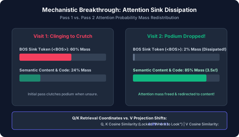
In standard LLMs, attention heads often dump 60%+ of their attention onto the very first token (the <BOS> or start token). Think of it like a nervous speaker clutching the podium—it’s an “attention crutch” used to store unneeded probability mass when the model is unsure where to look.

Here is the paper’s coolest mechanistic discovery:

In Pass 1: The model clings to the crutch (60% attention mass on the first token).
In Pass 2: Because the model already knows the context, it lets go of the podium. Attention on the first token drops to almost 2%, redirecting nearly 85% of its focus directly onto the actual code syntax, logical premises, and semantic demonstrations!

Plain-English Translation Cheat Sheet

Research Term in the Paper	What It Means in Plain English	Why You Should Care
Middle 50% Loop ( $r=2$ )	Re-running only the reasoning layers, skipping entry & exit.	Saves compute by only repeating where thinking happens.
Compute-Matched Trilemma	Balancing FLOPs, parameter storage, and KV cache memory.	Guarantees the model won’t cost more to train or serve.
$1/r = 0.5$ Residual Scaling	Halving the update size on looped layers.	Prevents math instability and numerical explosion.
Attention Sink Dissipation	Stopping attention from pooling uselessly at token #1.	Frees up attention bandwidth for actual code and logic.
Excess Residual ( $\delta_i$ )	Benchmark score above what validation loss predicts.	Proof that looping boosts true reasoning, not just memorization.

2. The Compute-Matching Trilemma: Reconciling Budget Trade-Offs

When comparing an unlooped baseline with a looped Transformer, three distinct physical resources dictate real-world deployment viability. Hiding or inflating any of these three invalidates the comparison:

$\text{1. Active Compute Budget:} \quad C_{\text{token}} \propto L_{\text{exec}} \cdot H^2 + \text{MoE Top-}k \text{ FLOPs}$

$\text{2. Knowledge Capacity Budget:} \quad N_{\text{non-emb}} \approx L_{\text{phys}} \cdot (d_{\text{attn\_weights}} + E_{\text{total}} \cdot d_{\text{expert\_weights}})$

$\text{3. Serving Memory Budget:} \quad M_{\text{KV}} \propto L_{\text{exec}} \cdot N_{\text{kv\_heads}} \cdot d_{\text{head}} \cdot N_{\text{ctx}}$

The Compute-Matching Trilemma: Dense vs SMELT MoE Looping

                          THE THREE BUDGET CONSTRAINTS
                          
           Per-Token FLOPs (C_token) <---> [Training & Inference Cost]
                        /                                \
                       /                                  \
                      v                                    v
Total Parameters (N_non-emb) <---------------> KV Cache Footprint (M_KV)
 [Knowledge & Memorization]                     [Serving Context Length]

Why Dense Looping Fails Under Compute Matching

In a standard dense Transformer, active FLOPs per token scale as $\mathcal{O}(L \cdot H^2)$ and total non-embedding parameters scale as $\mathcal{O}(L \cdot H^2)$ .

If you execute $L_{\text{exec}} = 1.5 \times L_{\text{phys}}$ by looping, per-token FLOPs grow by $50\%$ .
To bring per-token FLOPs back down to $1.0\times$ , you MUST shrink $H$ by a factor of $\sqrt{1 / 1.5} \approx 0.816$ .
However, in a dense network, shrinking $H$ to $0.816 H$ automatically shrinks stored parameter capacity $N_{\text{total}}$ to $(0.816)^2 \approx 66.7\%$ of the baseline!
The Dense Dilemma: You gain effective execution depth, but you permanently lose $33.3\%$ of your model’s knowledge capacity. In dense models, the parameter loss outweighs the depth gain.

How Sparse MoE Acts as the Parameter Decoupling Engine

Sparse Mixture-of-Experts breaks the coupling between per-token active FLOPs and total stored parameters. In an MoE layer:

Active FLOPs per token are determined ONLY by the top- $k$ selected experts ( $k=8$ active experts).
Total parameters are determined by the total pool of stored experts ( $E_{\text{total}}$ ).

SMELT leverages this decoupling seamlessly:

Narrow Hidden Dimension $H$ : To pay for re-executing the middle $50\%$ of layers twice ( $r=2$ ), SMELT reduces $H$ (e.g., from $1280 \rightarrow 1056$ at the 200M scale). This brings per-token active FLOPs back to parity ( $\le 3.9\%$ mismatch).
Expand Total Expert Count $E$ : Narrowing $H$ reduces the parameter count of each individual expert. SMELT compensates by increasing the total expert pool $E_{\text{total}}$ (e.g., from $192 \rightarrow 288$ experts per layer at 200M). Total stored parameters remain identical to the baseline ( $\le 1.0\%$ mismatch).
Adjust GQA Geometry: Head dimension $d_k$ is calibrated across the $1.5\times$ executed passes ( $L_{\text{exec}}$ ) so that total serving KV cache memory remains matched within $\le 3.6\%$ .

3. Dual-Level Mathematical Rigor

3.1 Intuitive Engineering Arithmetic

To understand how SMELT executes 18 effective layers on a 12-layer physical budget without extra FLOPs or KV memory, let us walk step-by-step through the 200M Scale, $S \approx 95\%$ Sparsity Cell:

Parameter / Metric	Baseline (Unlooped MoE)	SMELT (Looped MoE)	Mismatch / Delta
Physical Layers ( $L_{\text{phys}}$ )	12 layers	12 layers	$0\%$
Loop Configuration	Unlooped ( $r=1$ )	Middle 50% ( $L_4 \dots L_9$ ) $\times 2$	$+6$ exec passes
Executed Depth ( $L_{\text{exec}}$ )	12 layers	18 layers	$+50\%$ depth
Hidden Dimension ( $H$ )	1280	1056	$-17.5\%$ width
Expert Pool / Layer ( $E_{\text{total}}$ )	192 total (8 active)	288 total (8 active)	$+50.0\%$ experts
Active Params / Traversal	0.209B	0.142B	$-32.0\%$
Total Stored Params ( $N_{\text{total}}$ )	3.87B	3.89B	$+0.4\%$
Per-Token Training FLOPs ( $F$ )	$1.33 \times 10^9$	$1.37 \times 10^9$	$+2.9\%$
KV Cache Footprint / Token	$1.00\times$ Baseline	$1.031\times$ Baseline	$+3.1\%$

Key Takeaway: An engineering leader sees a model executing 18 layers of deep computational reasoning per token while incurring zero parameter bloat, zero VRAM penalty, and under $+2.9\%$ FLOP equivalence!

3.2 Formal FLOP & Parameter Accounting

Forward & Backward FLOP Accounting per Token

For sequence length $N_{\text{ctx}}$ , hidden dimension $H$ , query heads $N_Q$ , key/value heads $N_{\text{KV}}$ , head dimension $d_k$ , active experts $k$ , total experts $E_{\text{total}}$ , and expert intermediate dimension $d_{\text{ffn}}$ , the exact single-pass forward FLOPs per token across $L_{\text{exec}}$ executed layers is:

$F_{\text{forward}} = L_{\text{exec}} \cdot \left[ \underbrace{2H(N_Q d_k + 2 N_{\text{KV}} d_k + N_Q d_k)}_{\text{Q, K, V, O projections}} + \underbrace{4 N_Q N_{\text{ctx}} d_k}_{\text{Attention Scores and Context}} + \underbrace{2H E_{\text{total}}}_{\text{Router Gating}} + \underbrace{4 k H d_{\text{ffn}}}_{\text{Top-}k \text{ MoE FFN}} \right]$

$F_{\text{train}} \approx 3 \cdot F_{\text{forward}} \quad (1 \text{ forward pass} + 2 \text{ backward passes})$

FLOP Parity Under Looping

When SMELT executes $L_{\text{exec}} = 1.5 L_{\text{phys}}$ passes by looping the middle $50\%$ of layers twice ( $r=2$ ), active per-token FLOPs are held equal by narrowing the hidden dimension $H_{\text{smelt}} < H_{\text{base}}$ , satisfying:

$F_{\text{SMELT\_train}} \approx F_{\text{base\_train}} \quad (\le 3.9\% \text{ residual error across all grid cells})$

By selecting $H_{\text{smelt}} < H$ and $E_{\text{smelt}} > E_{\text{base}}$ , SMELT enforces:

$F_{\text{SMELT\_train}} \approx F_{\text{base\_train}} \quad (\text{within } \le 3.9\% \text{ residual error})$

3.3 Residual Stream Variance Mechanics & The $1/r$ Rule

In weight-tied recurrent passes, naively executing $\mathbf{x}^{(t)} = \mathbf{x}^{(t-1)} + \mathcal{F}(\mathbf{x}^{(t-1)})$ causes severe numerical instability. Because the transformation weights $\mathbf{W}$ in $\mathcal{F}(\cdot)$ are identical across visits, residual updates $\Delta \mathbf{x}^{(1)}$ and $\Delta \mathbf{x}^{(2)}$ exhibit high positive cross-covariance:

$\text{Cov}\left( \Delta \mathbf{x}^{(1)}, \Delta \mathbf{x}^{(2)} \right) > 0$

Without compensation, the residual variance inflates quadratically across recurrent visits:

$\text{Var}\left( \mathbf{x}^{(r)} \right) = \text{Var}(\mathbf{x}^{(0)}) + \sum_{t=1}^r \text{Var}\left( \mathcal{F}(\mathbf{x}^{(t-1)}) \right) + 2 \sum_{i < j} \text{Cov}\left( \mathcal{F}(\mathbf{x}^{(i)}), \mathcal{F}(\mathbf{x}^{(j)}) \right)$

This variance inflation causes pre-norm inputs to explode before RMSNorm, leading to gradient explosion during backpropagation through depth.

                              RESIDUAL STREAM STABILITY
                              
Unscaled Loop (1.0x):  x_0 ------> [+] ------> [+] ------> Explosion / Drift!
                                    ^           ^
                                    |           |
                                 F(x_0)      F(x_1) [Correlated Updates]

Scaled Loop (1/r = 0.5x): x_0 ---> [+] ------> [+] ------> Stable Variance Trajectory
                                    ^           ^
                                    |           |
                                0.5*F(x_0)  0.5*F(x_1)

The SMELT Resolution

SMELT dampens every sub-layer residual update within the looped segment by $\frac{1}{r}$ (where $r=2$ , scaling factor $= 0.5$ ):

$\mathbf{x}_{l}^{(t)} = \mathbf{x}_{l}^{(t-1)} + \frac{1}{r} \mathcal{F}_l\left( \mathbf{x}_{l}^{(t-1)} \right)$

Explicitly, inside the looped middle span: $\mathbf{x}_{\text{attn}} = \mathbf{x}_{\text{in}} + \frac{1}{r} \text{Attention}\left( \text{RMSNorm}(\mathbf{x}_{\text{in}}) \right)$

$\mathbf{x}_{\text{out}} = \mathbf{x}_{\text{attn}} + \frac{1}{r} \text{MoE}\left( \text{RMSNorm}(\mathbf{x}_{\text{attn}}) \right)$

This $0.5\times$ factor bounds the variance expansion rate $\frac{d}{dt} \text{Var}(\mathbf{x}^{(t)})$ , ensuring gradient norm stability across repeated backpropagation paths.

3.4 Chinchilla Scaling Law Formulation & Fitted Exponents

To evaluate whether SMELT achieves a fundamental algorithmic advance over standard MoE Transformers, Wang et al. fit separate Chinchilla-style scaling surfaces across 144 sparse training checkpoints spanning $1.3 \times 10^{19}$ to $2.2 \times 10^{21}$ total training FLOPs.

Parametric Form

Replacing standard parameter count $N$ with active per-token FLOPs $F$ and compute-equivalent sparsity $S = 1 - \frac{N_{\text{act}}^{\text{eq}}}{N}$ :

$L(F, S, D) = \mathcal{L}_0 + \frac{A (1 - S)^b}{F^a} + \frac{K}{D^c}$

$\mathcal{L}_0$ : Irreducible loss floor (nats) [renamed from $E$ to avoid confusion with expert count $E_{\text{total}}$ ].
$F$ : Measured per-token training FLOPs.
$S$ : Compute-equivalent sparsity level ( $S \in \{85\%, 95\%, 97\%\}$ ).
$D$ : Cumulative training tokens.

Huber-Loss Optimization

Both surfaces were fitted independently using Huber-loss ( $\delta = 10^{-3}$ ) minimization on log-loss with L-BFGS-B optimization:

Architecture	Floor ( $\mathcal{L}_0$ )	Capacity ( $A$ )	Data ( $K$ )	Cap Exp ( $a$ )	Sparsity Exp ( $b$ )	Data Exp ( $c$ )	Fit RMSE
Baseline (MoE)	1.4439	$1.366 \times 10^3$	$1.975 \times 10^6$	0.3703	0.1530	0.6594	0.00554 nats
SMELT (Ours)	1.4493	$1.963 \times 10^3$	$5.264 \times 10^6$	0.3892	0.1460	0.7011	0.00952 nats

Derivation of the Compute-Optimal Frontier Exponent $\gamma$

Balancing capacity FLOPs $F^*$ and token count $D^* = C / F^*$ yields the compute-optimal loss trajectory:

$L^*(C, S) = \mathcal{L}_0 + \text{Prefactor}(S) \cdot C^{-\gamma}, \quad \text{where } \gamma = \frac{a \cdot c}{a + c}$

$\gamma_{\text{Baseline}} = \frac{0.3703 \times 0.6594}{0.3703 + 0.6594} = \mathbf{0.2371}$

$\gamma_{\text{SMELT}} = \frac{0.3892 \times 0.7011}{0.3892 + 0.7011} = \mathbf{0.2502} \quad (+5.5\% \text{ steeper drop!})$

Compute Efficiency Gain (CE Gain) Derivation

CE Gain measures the percentage of training compute SMELT saves over the baseline to hit identical validation loss:

$\text{CE Gain} = 1 - \frac{C_{\text{SMELT}}}{C_{\text{Baseline}}}$

Training FLOP Budget ( $C$ )	$S \approx 85\%$ Sparsity	$S \approx 95\%$ Sparsity	$S \approx 97\%$ Sparsity
$10^{20}$ FLOPs	10.0% [1, 22]	7.8% [3, 15]	6.8% [4, 14]
$10^{21}$ FLOPs	18.0% [8, 28]	15.8% [10, 25]	14.7% [8, 25]
$10^{22}$ FLOPs (Extrapolated)	23.5% [8, 42]	20.9% [0, 48]	19.6% [0, 51]
Brackets show 95% confidence intervals from 2,000 cell-bootstrap draws.

4. Architectural Deep-Dive & Visual Schematics

4.1 Architecture Flow & Layer Placement

SMELT adopts a Prelude-Recur-Coda layout. For a physical depth $L$ , the middle $50\%$ span $m = L/2$ loops twice ( $r=2$ ), flanked by unshared entry and exit layers:

SMELT Stack Execution Trace

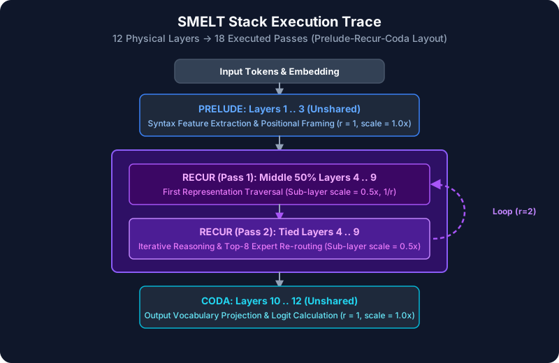
                      SMELT STACK EXECUTION TRACE (L_phys = 12, L_exec = 18)
                      
   Input Tokens
        |
   +----+----+
   | Embed   |
   +----+----+
        |
[PRELUDE: Unlooped Entry]
   Layer 1  (r=1, scale=1.0)
   Layer 2  (r=1, scale=1.0)
   Layer 3  (r=1, scale=1.0)
        |
[RECUR: Looped Middle 50% Block] <-----------------------+
   Layer 4  (Pass 1, scale=0.5)                          |
   Layer 5  (Pass 1, scale=0.5)                          |
   Layer 6  (Pass 1, scale=0.5)                          |
   Layer 7  (Pass 1, scale=0.5)                          |
   Layer 8  (Pass 1, scale=0.5)                          |
   Layer 9  (Pass 1, scale=0.5)                          |
        |                                                | Loop Iteration (r=2)
        +------------------------------------------------+
        |
   Layer 4  (Pass 2, scale=0.5)  <-- Re-uses tied weights, re-routes experts
   Layer 5  (Pass 2, scale=0.5)
   Layer 6  (Pass 2, scale=0.5)
   Layer 7  (Pass 2, scale=0.5)
   Layer 8  (Pass 2, scale=0.5)
   Layer 9  (Pass 2, scale=0.5)
        |
[CODA: Unlooped Exit]
   Layer 10 (r=1, scale=1.0)
   Layer 11 (r=1, scale=1.0)
   Layer 12 (r=1, scale=1.0)
        |
   +----+----+
   | RMSNorm |
   +----+----+
        |
   LM Head Output

Mermaid Schematic

graph TD
    A[Token Input] --> B[Embedding Layer]
    B --> C[Prelude: Layers 1..3<br/>Unshared, scale=1.0]
    C --> D[Recur Pass 1: Layers 4..9<br/>Shared Weights, scale=0.5]
    D --> E[Recur Pass 2: Layers 4..9<br/>Shared Weights, scale=0.5]
    E --> F[Coda: Layers 10..12<br/>Unshared, scale=1.0]
    F --> G[Final RMSNorm & LM Head]

4.2 Design Space Ablations

To isolate why SMELT succeeds, Wang et al. executed three rigorous hyperparameter sweeps at the 200M scale:

Ablation Axis	Sweep Range	Optimal Choice	Mechanistic Rationale
1. Loop Span ( $m / L$ )	0% (Base) to 100% (Full)	Middle 50% Span	Early layers handle syntax extraction; final layers project to vocabulary. Middle layers thrive on iteration.
2. Depth-to-Width Ratio	$L_{\text{phys}} \in \{9, 12, 15, 18\}$	$L_{\text{phys}}=12$ ( $L_{\text{exec}}=18$ )	Shared middle layers receive multi-depth gradient signals, making extra depth easier to optimize.
3. Loop Count ( $r$ )	$r \in \{1, 2, 3, 4\}$	$r = 2$ Passes	$r \ge 3$ forces $H$ to become too thin under matched FLOP budget caps, degrading performance.

4.3 Mechanistic Interpretability: Inside the Second Pass

Why does visiting the same physical layers a second time produce superior representations? The paper probes the internal activations on a 1M-token validation sample across four dimensions:

Attention Sink Dissipation & Value Projection Shifts

Probe Axis	Empirical Observation	Functional Interpretation
1. Attention Sink Dissipation	Segment-start BOS attention mass drops from 0.60 (Visit 1) to 0.02 (Visit 2).	Second visit clears uninformative sink mass and redirects attention to content tokens.
2. $Q/K$ vs. $V$ Projections	$Q, K$ cosine similarity = 0.89–0.93; $V$ cosine similarity drops to 0.65–0.74.	Model retains retrieval coordinates (“where to look”) while updating semantic content (“what to read”).
3. Expert Routing Overlap	Reuses 2–3 core experts out of 8 selected; diversifies remaining 5–6 experts.	Maintains core functional routing while expanding expert representation capacity.
4. Residual Write Alignment	$\\|\Delta x^{(2)}\\| / \\|\Delta x^{(1)}\\| = 1.2\times - 3.5\times$ ; pairwise cosine similarity = 0.42–0.65.	Visit 2 amplifies and aligns with Visit 1 signal rather than overwriting it.

                        ATTENTION SINK REDISTRIBUTION (Visit 1 vs. Visit 2)
                        
   Visit 1 (Initial Pass):   [BOS / Sink Token] =====( 60% Mass )=====> Heavy Concentration
                             [Content Tokens  ] -----( 24% Mass )-----> Starved Attention
                             
   Visit 2 (Recurrent Pass): [BOS / Sink Token] --( 2% Mass )---------> Dissipated!
                             [Content Tokens  ] =====( 85% Mass )=====> Massively Amplified!

5. PyTorch Reference Implementation & Structural Walkthrough

Below is a clean, executable PyTorch reference implementation of the SMELT Architecture, featuring Grouped-Query Attention (GQA), Top-8 Sparse MoE routing with auxiliary load-balancing loss, RMSNorm, physical layer parameterization, middle 50% looping ( $r=2$ ), and $\frac{1}{r} = 0.5$ residual scaling.

[!NOTE]
Systems Disclaimer: The implementation below serves as a structural reference for architectural clarity. Production LLM serving runtimes (such as Megablocks, vLLM, TensorRT-LLM, or Triton fused kernels) replace the educational Python for-loop over experts with optimized grouped GEMM routines (grouped_gemm) to avoid CPU-GPU launch overhead.

import math
import torch
import torch.nn as nn
import torch.nn.functional as F
from typing import Optional, Tuple, Dict

class RMSNorm(nn.Module):
    """Root Mean Square Layer Normalization."""
    def __init__(self, dim: int, eps: float = 1e-6):
        super().__init__()
        self.eps = eps
        self.weight = nn.Parameter(torch.ones(dim))

    def forward(self, x: torch.Tensor) -> torch.Tensor:
        variance = x.pow(2).mean(-1, keepdim=True)
        return x * torch.rsqrt(variance + self.eps) * self.weight

class TopKMoE(nn.Module):
    """
    Top-K Sparse Mixture-of-Experts (MoE) FFN with Load-Balancing Loss.
    """
    def __init__(self, d_model: int, num_experts: int, top_k: int, ffn_dim: int):
        super().__init__()
        self.num_experts = num_experts
        self.top_k = top_k
        self.gate = nn.Linear(d_model, num_experts, bias=False)
        self.experts = nn.ModuleList([
            nn.Sequential(
                nn.Linear(d_model, ffn_dim, bias=False),
                nn.SiLU(),
                nn.Linear(ffn_dim, d_model, bias=False)
            ) for _ in range(num_experts)
        ])

    def forward(self, x: torch.Tensor) -> Tuple[torch.Tensor, torch.Tensor]:
        B, T, C = x.shape
        x_flat = x.view(-1, C) # (B*T, C)
        
        router_logits = self.gate(x_flat) # (B*T, num_experts)
        routing_weights = F.softmax(router_logits, dim=-1)
        
        weights, selected_experts = torch.topk(routing_weights, self.top_k, dim=-1)
        weights = weights / weights.sum(dim=-1, keepdim=True) # Normalize top-k weights

        out = torch.zeros_like(x_flat)
        for i in range(self.num_experts):
            mask = (selected_experts == i)
            if mask.any():
                batch_idx, topk_idx = torch.where(mask)
                token_inputs = x_flat[batch_idx]
                expert_out = self.experts[i](token_inputs)
                expert_weights = weights[batch_idx, topk_idx].unsqueeze(-1)
                out.index_add_(0, batch_idx, expert_out * expert_weights)

        # Compute auxiliary load-balancing loss (Switch Transformer formulation)
        density_1 = routing_weights.mean(dim=0)
        tokens_per_expert = torch.zeros(self.num_experts, device=x.device)
        for i in range(self.num_experts):
            tokens_per_expert[i] = (selected_experts == i).sum().float()
        density_2 = tokens_per_expert / (B * T * self.top_k)
        aux_loss = self.num_experts * torch.sum(density_1 * density_2)

        return out.view(B, T, C), aux_loss

class GroupedQueryAttention(nn.Module):
    """
    Grouped-Query Attention (GQA) with dual-pass KV-caching support.
    """
    def __init__(self, d_model: int, num_heads: int, num_kv_heads: int, head_dim: int):
        super().__init__()
        self.num_heads = num_heads
        self.num_kv_heads = num_kv_heads
        self.head_dim = head_dim
        self.num_queries_per_kv = num_heads // num_kv_heads

        self.q_proj = nn.Linear(d_model, num_heads * head_dim, bias=False)
        self.k_proj = nn.Linear(d_model, num_kv_heads * head_dim, bias=False)
        self.v_proj = nn.Linear(d_model, num_kv_heads * head_dim, bias=False)
        self.out_proj = nn.Linear(num_heads * head_dim, d_model, bias=False)

    def forward(
        self, 
        x: torch.Tensor, 
        mask: Optional[torch.Tensor] = None,
        layer_kv_cache: Optional[Tuple[torch.Tensor, torch.Tensor]] = None
    ) -> Tuple[torch.Tensor, Tuple[torch.Tensor, torch.Tensor]]:
        B, T, _ = x.shape
        q = self.q_proj(x).view(B, T, self.num_heads, self.head_dim).transpose(1, 2)
        k = self.k_proj(x).view(B, T, self.num_kv_heads, self.head_dim).transpose(1, 2)
        v = self.v_proj(x).view(B, T, self.num_kv_heads, self.head_dim).transpose(1, 2)

        if layer_kv_cache is not None:
            k_prev, v_prev = layer_kv_cache
            k = torch.cat([k_prev, k], dim=-2)
            v = torch.cat([v_prev, v], dim=-2)
        updated_kv = (k, v)

        if self.num_queries_per_kv > 1:
            k_expanded = k.repeat_interleave(self.num_queries_per_kv, dim=1)
            v_expanded = v.repeat_interleave(self.num_queries_per_kv, dim=1)
        else:
            k_expanded, v_expanded = k, v

        scores = torch.matmul(q, k_expanded.transpose(-2, -1)) / math.sqrt(self.head_dim)
        if mask is not None:
            scores = scores + mask

        attn_weights = F.softmax(scores, dim=-1)
        output = torch.matmul(attn_weights, v_expanded).transpose(1, 2).contiguous().view(B, T, -1)
        return self.out_proj(output), updated_kv

class SMELTBlock(nn.Module):
    def __init__(self, d_model: int, num_heads: int, num_kv_heads: int, head_dim: int, num_experts: int, top_k: int, ffn_dim: int):
        super().__init__()
        self.norm1 = RMSNorm(d_model)
        self.attn = GroupedQueryAttention(d_model, num_heads, num_kv_heads, head_dim)
        self.norm2 = RMSNorm(d_model)
        self.moe = TopKMoE(d_model, num_experts, top_k, ffn_dim)

    def forward(
        self, 
        x: torch.Tensor, 
        scale: float = 1.0, 
        mask: Optional[torch.Tensor] = None,
        layer_kv_cache: Optional[Tuple[torch.Tensor, torch.Tensor]] = None
    ) -> Tuple[torch.Tensor, Tuple[torch.Tensor, torch.Tensor], torch.Tensor]:
        attn_out, updated_kv = self.attn(self.norm1(x), mask=mask, layer_kv_cache=layer_kv_cache)
        x = x + scale * attn_out
        moe_out, aux_loss = self.moe(self.norm2(x))
        x = x + scale * moe_out
        return x, updated_kv, aux_loss

class SMELTTransformer(nn.Module):
    """
    Decoder-Only Transformer implementing true Block Recurrence.
    Prelude (L1..L3) -> Recur Block (L4..L9 executed r=2 times) -> Coda (L10..L12)
    Stores dual-pass KV caches for all 18 executed layer passes.
    """
    def __init__(
        self,
        vocab_size: int = 32000,
        d_model: int = 1056,
        num_layers: int = 12,
        num_heads: int = 16,
        num_kv_heads: int = 4,
        head_dim: int = 55,   # Calibrated: 18 passes * 4 * 55 = 3960 (Baseline: 12 * 4 * 80 = 3840 -> 1.031x)
        num_experts: int = 288,
        top_k: int = 8,
        ffn_dim: int = 1056,
        loop_r: int = 2,
        loop_start_ratio: float = 0.25,
        loop_end_ratio: float = 0.75
    ):
        super().__init__()
        self.tok_embeddings = nn.Embedding(vocab_size, d_model)
        self.layers = nn.ModuleList([
            SMELTBlock(d_model, num_heads, num_kv_heads, head_dim, num_experts, top_k, ffn_dim)
            for _ in range(num_layers)
        ])
        self.norm_f = RMSNorm(d_model)
        self.lm_head = nn.Linear(d_model, vocab_size, bias=False)

        self.num_layers = num_layers
        self.loop_r = loop_r
        self.loop_start = int(num_layers * loop_start_ratio)  # Layer 4 (0-indexed: index 3)
        self.loop_end = int(num_layers * loop_end_ratio)      # Layer 10 (0-indexed: index 9, exclusive)
        self.loop_scale = 1.0 / loop_r                        # 0.5x scaling

    def forward(
        self, 
        input_ids: torch.Tensor, 
        mask: Optional[torch.Tensor] = None,
        kv_caches: Optional[List[Tuple[torch.Tensor, torch.Tensor]]] = None
    ) -> Tuple[torch.Tensor, torch.Tensor, List[Tuple[torch.Tensor, torch.Tensor]]]:
        h = self.tok_embeddings(input_ids)
        total_aux_loss = 0.0
        new_kv_caches = []
        cache_idx = 0

        # 1. PRELUDE: Layers 0 to loop_start - 1 (Unlooped, scale=1.0)
        for i in range(0, self.loop_start):
            c = kv_caches[cache_idx] if kv_caches is not None else None
            h, updated_c, aux = self.layers[i](h, scale=1.0, mask=mask, layer_kv_cache=c)
            total_aux_loss += aux
            new_kv_caches.append(updated_c)
            cache_idx += 1

        # 2. RECUR BLOCK: True Block Recurrence over loop_start to loop_end - 1
        for pass_idx in range(self.loop_r):
            for i in range(self.loop_start, self.loop_end):
                c = kv_caches[cache_idx] if kv_caches is not None else None
                h, updated_c, aux = self.layers[i](h, scale=self.loop_scale, mask=mask, layer_kv_cache=c)
                total_aux_loss += aux
                new_kv_caches.append(updated_c)
                cache_idx += 1

        # 3. CODA: Layers loop_end to num_layers - 1 (Unlooped, scale=1.0)
        for i in range(self.loop_end, self.num_layers):
            c = kv_caches[cache_idx] if kv_caches is not None else None
            h, updated_c, aux = self.layers[i](h, scale=1.0, mask=mask, layer_kv_cache=c)
            total_aux_loss += aux
            new_kv_caches.append(updated_c)
            cache_idx += 1

        logits = self.lm_head(self.norm_f(h))
        return logits, total_aux_loss, new_kv_caches

6. Empirical Results & Benchmark Dissection

6.1 Full Grid Configurations & Scale Breakdown

Representative configurations across the 4 primary active parameter scales (evaluated at the key $\approx 95\%–97\%$ sparsity level from the full 16-cell grid):

Scale	Arch	$H$	$L_{\text{phys}}$	GQA ( $N_Q / N_{\text{KV}} / d_k$ )	Experts (Tot/Act)	Active Params	Sparsity ( $S$ )	Total Params	FLOP Ratio	KV Ratio
100M	Baseline	672	10	12 / 4 / 56	336 / 8	0.102B	97.2%	3.70B	1.000	1.000
	SMELT	576	10	12 / 4 / 36	504 / 8	0.070B	97.4%	3.70B	1.039	0.964
200M	Baseline	1280	12	16 / 4 / 80	192 / 8	0.209B	94.6%	3.87B	1.000	1.000
	SMELT	1056	12	16 / 4 / 55	288 / 8	0.142B	94.7%	3.89B	1.029	1.031
600M	Baseline	1792	20	28 / 7 / 64	336 / 8	0.675B	96.9%	21.83B	1.000	1.000
	SMELT	1512	20	28 / 7 / 42	504 / 8	0.459B	96.9%	21.70B	1.031	0.984
1.6B	Baseline	2304	30	36 / 9 / 64	336 / 8	1.651B	96.9%	53.89B	1.008	1.000
	SMELT	1848	30	36 / 9 / 42	504 / 8	1.103B	97.0%	53.90B	1.008	0.984

Note: SMELT shrinks KV channel width per physical layer ( $N_{\text{KV}} \cdot d_k$ ) by $\sim 31\%$ , holding total serving KV memory ( $M_{\text{KV}}$ ) equal to the baseline across all 18 executed layer passes.

6.2 Downstream Benchmark Win Rates & Excess Residual Calibration

On downstream evaluations across 96 matched Baseline/SMELT pairs:

DCLM Completion (Gold-Completion Micro Loss): SMELT wins 96 out of 96 matched pairs (100% win rate).
DCLM Core (22-Task Suite Centered Accuracy): SMELT wins 83 out of 96 matched pairs (86.5% win rate).
MMLU 5-Shot Accuracy: SMELT wins 29 out of 30 matched pairs whose baseline scores at least 10% above chance.

Monotone Sigmoid Calibration & Excess Residual $\delta_i$

To test whether downstream gains are merely proportional to validation loss reduction or exceed it, Wang et al. fit a monotone sigmoid calibration mapping validation loss $\ell$ to benchmark accuracy $\hat{y}(\ell)$ :

$\hat{y}(\ell) = b + \frac{a}{1 + \exp\left[ -d \cdot \alpha (\ell - \tau) \right]}$

The downstream excess residual $\delta_i = y_i - \hat{y}(\ell_i)$ measures the net benchmark advantage beyond what validation loss predicts:

Model Scale	DCLM Completion Residual (mn)	DCLM Core Residual (pp)	MMLU Residual (pp)
100M Scale	+1.7 mn	+0.5 pp	+0.3 pp
200M Scale	+6.5 mn	+0.9 pp	+1.0 pp
600M Scale	+11.6 mn	+1.0 pp	+2.2 pp
1.6B Scale	+12.3 mn	+1.2 pp	+1.6 pp
Pooled (All)	+8.0 mn	+0.9 pp	+1.3 pp
Note: Excess residual grows monotonically with scale, proving that looping provides structural reasoning benefits that expand at scale!

6.3 Domain-Specific Gains & In-Context Learning (ICL) Amplification

Per-Domain Compute Efficiency Gain

Restricting the scaling surface to specific validation categories at $C = 10^{21}$ FLOPs and $S \approx 95\%$ :

Code: 20.4% CE Gain (Highest gain due to strict syntactic dependency & long-range structure).
Finance: 16.8% CE Gain
Math/STEM: 16.6% CE Gain
World Knowledge: 14.9% CE Gain
Web Text: 14.8% CE Gain

Sample Length & In-Context Learning (ICL) Amplification

Long Contexts: SMELT’s normalized loss gain on long documents (512–4096 tokens) is 1.52x higher than on short documents (32–256 tokens). Baseline controls (adding parameters or adding experts) show flat profiles (0.98x and 0.88x).
In-Context Demonstrations: Few-shot accuracy gap widens from 0.9 pp at $k=0$ shots to 1.9 pp at $k=1..8$ shots.
Dyck Language Bracket Matching: On demonstration-sensitive exact-match Dyck tasks, SMELT’s accuracy gap expands continuously with shot count, reaching 29.8% vs. 26.4% at $k=32$ shots!

                        ICL ACCURACY EXPANSION (Dyck Languages)
                        
Accuracy (%)
  30% |                                                    * (29.8% SMELT)
      |                                           *-------
  25% |                                   *------- o (26.4% Baseline)
      |                          *-------- o------
  20% |                 *-------- o-------
      |        *-------- o--------
   0% |--------o---------
      +-------------------------------------------------------------------> Shots (k)
              k=0       k=1      k=4       k=8      k=16     k=32

7. Systems Engineering, Serving & Production Trade-Offs

For AI Infrastructure leads, VLLM kernel developers, and CTOs evaluating deployment feasibility, SMELT presents a clean operational profile:

Production Phase	Baseline MoE	SMELT MoE	Systems Impact & Analysis
1. Prefill Phase (Prompt Compute)	Compute-Bound (GEMM) $1.0\times$ FLOPs	Compute-Bound (GEMM) $1.0\times$ FLOPs	Identical TTFT. Per-token FLOP matching ensures zero prefill slowdown.
2. Decoding Phase (Token Generation)	Memory-Bandwidth Bound (HBM Parameter Read)	Memory-Bandwidth Bound (HBM Parameter Reuse)	Reuses total stored parameter footprint in HBM, but 6-layer block exceeds GPU L2 cache capacity.
3. KV Cache VRAM (Serving Context)	$1.0\times$ Baseline VRAM	$1.031\times$ Baseline VRAM	Stores 18 effective KV cache passes, but $31.3\%$ per-layer channel width reduction maintains VRAM parity.

7.1 Prefill vs. Decoding Latency & Memory Bandwidth Dynamics

Prefill (Prompt Processing - Compute-Bound): Prefill processing is strictly compute-bound by GEMM throughput. Because SMELT matches active per-token FLOPs within $\le 3.9\%$ , Time-To-First-Token (TTFT) remains virtually identical to the unlooped baseline.
Decoding (Auto-regressive Generation - Memory-Bandwidth Bound): Single-token decoding is memory-bandwidth bound by High Bandwidth Memory (HBM) parameter read throughput.
- L2 Cache Capacity Check: In block-level recurrence over a 6-layer block ( $L_4 \dots L_9$ ), the repeated parameter footprint ( $\\approx 3.9\text{ GB}$ stored / $\approx 840\text{ MB}$ active top-8 weights at 200M scale) far exceeds the GPU L2 cache capacity (50 MB on Nvidia H100 SXM, 120 MB on B200). Therefore, weight persistence across block passes in L2 cache does not occur.
- HBM Read & Arithmetic Intensity: SMELT’s true systems advantage during decoding comes from storing fewer unique physical parameter bytes in HBM while executing higher arithmetic intensity (higher $\text{FLOPs} / \text{Byte}$ ). Because SMELT stores identical total parameter bytes to the unlooped baseline ( $N_{\text{total}} \le 1.0\%$ mismatch), HBM parameter traffic per generated token remains matched.

7.2 Dual-Pass KV Cache Footprint Mechanics

18 Effective Cache Layers: During auto-regressive decoding of token $t$ , the second pass of Layer 4 operates on updated residual states $\mathbf{h}_t^{(2)}$ output from Layer 9 (Pass 1). Consequently, Layer 4 produces distinct key/value projections ( $K^{(2)}, V^{(2)}$ ) on Pass 2. To preserve causal attention across both passes, runtimes must store 18 effective sets of KV caches ( $3 + 6 \times 2 + 3$ ).
GQA Channel Calibration: To maintain $1.0\times$ serving KV memory parity ( $M_{\text{KV}} \le 3.6\%$ mismatch), SMELT shrinks the KV channel width per physical layer ( $N_{\text{KV}} \cdot d_k$ ) by $\approx 31.3\%$ (e.g., reducing $N_{\text{KV}}$ from 4 to 2 or shrinking head dimension $d_k$ ). This calibration ensures that 18 effective KV cache passes consume identical total VRAM byte capacity to the 12-layer unlooped baseline.

7.3 CUDA/Triton Kernel Locality

The sequential execution dependency of recurrent pass 2 on pass 1 prevents intra-token layer parallelism. However, Triton/CUDA kernels handling MoE top-8 routing benefit from shared gate parameters across visits, lowering overall kernel launch overhead relative to a physically twice-as-deep unlooped model.

8. Strategic Takeaways for AI Engineering Leaders

#	Actionable Engineering Lesson	Strategic Implementation
1	Enforce Trilemma Budget Matching	Never evaluate looped models on parameter count alone. Always hold per-token FLOPs, total stored parameters, and KV cache footprint strictly equal.
2	Use MoE as Capacity Recovery Engine	Dense looping fails because narrowing $H$ destroys parameters. Sparse MoE recovers parameter capacity by expanding expert count $E$ while keeping top- $k$ FLOPs locked.
3	Loop Middle 50% Twice at 0.5x Scale	Keep unshared entry/exit layers for syntax/vocabulary projections. Scale recurrent sub-layer updates by $1/r = 0.5$ to ensure residual stream stability.
4	Capitalize on Code & Long-Context ICL	SMELT’s second pass dissipates attention sinks and enhances retrieval, yielding peak compute savings (20.4%) on code and multi-shot reasoning tasks.

Technical Analysis completed based on arXiv:2609.01343 (“SMELT: Scaling Laws for Compute-Matched MoE Looped Transformers” by Shaowen Wang et al., ByteDance Seed & Tsinghua University).